Explicit Lifting
Explicit lifting is a feature of GoodData’s Extensible Analytics Engine that grants you greater flexibility in aggregating metrics in reports.
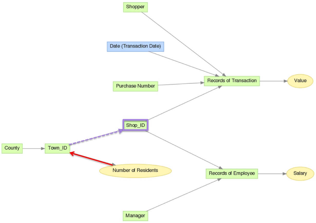
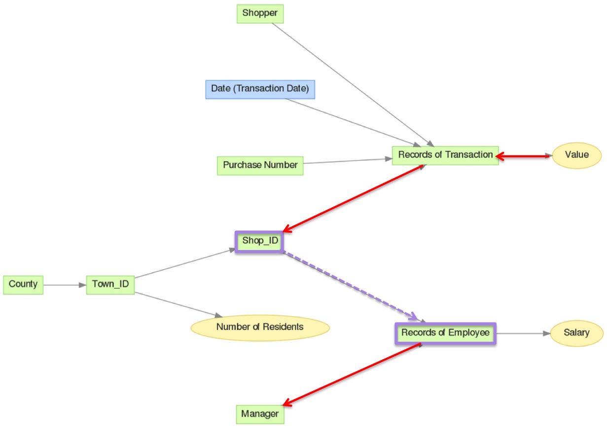
In the logical data model diagram (LDM) below, metrics aggregated from the Value fact, such as SELECT SUM(Value), can be aggregated by any of the attributes in red. Notice that these are the attributes with arrows that point to Value.
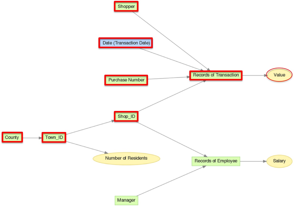
With explicit lifting you can traverse against the grain of aggregation using the BY keyword to lock the aggregation level at an attribute that would otherwise not be able to slice a particular metric.
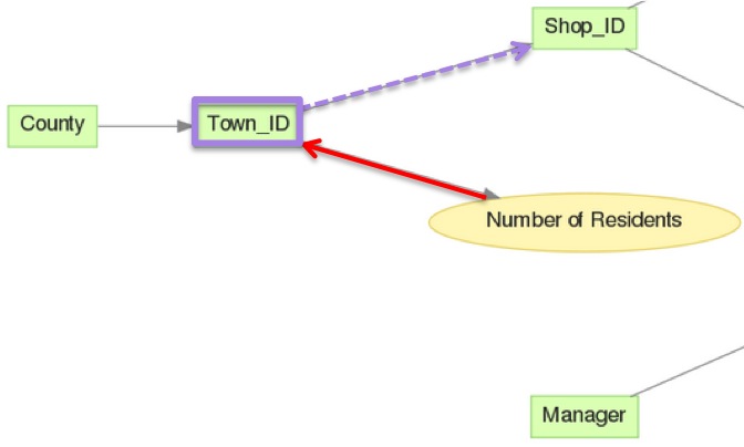
In the following example in the same LDM, see how explicit lifting allows you to slice the Number of Residents metric by Shop_ID, even though Shop_ID does not appear to be related to the Number of Residents fact.
This aggregation is described in greater detail in Example 1 below.
Example 1 - Lifting one aggregation level
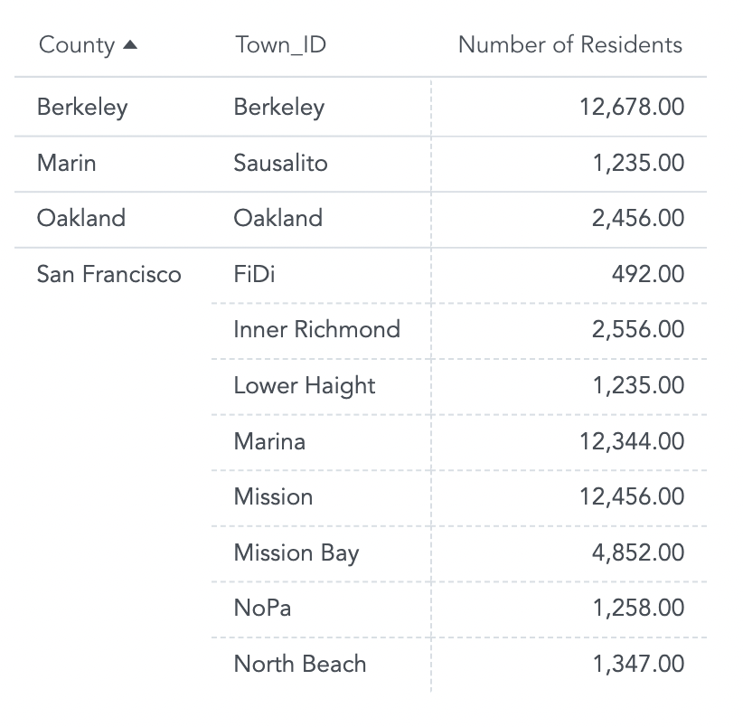
The following metric represents the total number of residents in a town.
SELECT SUM(Number of Residents)
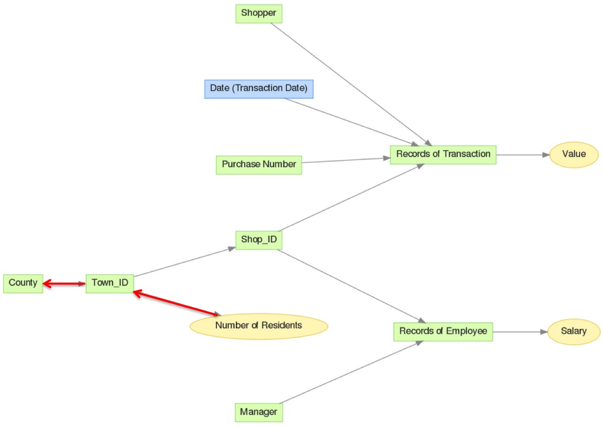
In the project’s LDM, displayed below, you can see that Number of Residents metric can be sliced by town (Town_ID) or by county (County).
The resulting report looks like the following:
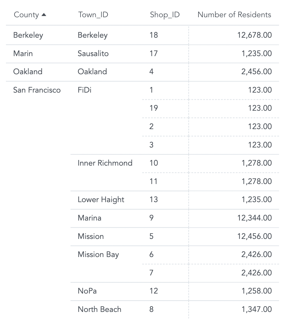
With explicit lifting, you can slice metrics by other attributes that are not directly related to the metric’s foundational fact. For example, you can modify its definition to slice the Number of Residents metric by Shop_ID.
SELECT SUM(Number of Residents) BY Shop_ID
The report now shows the Number of Residents in the town where each shop is located. The metric is aggregated at the Town_ID level.
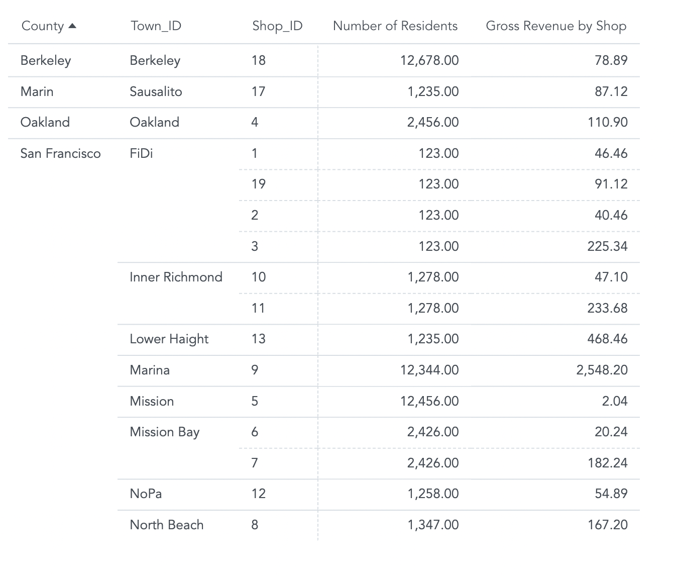
Now you can compare the Number of Residents metric side by side with a metric that represents the gross revenue of each shop (i.e. the total value of all transactions aggregated at the Shop_ID level).
To count the gross revenue, create the following metric:
SELECT SUM(Value)
You can break this metric down by any related attribute of larger granularity (see red attributes in first graphic, above) by adding those attributes at the report level.
For example, add County, Town_ID, and Shop_ID attributes to the report. This allows you to look for correlations between number of residents in the town in which a shop is located, and the gross revenue of each shop.
For a closer look at the correlation between the two metrics, remove the County and Town_ID attributes from the report and visualize the modified report as a scatter chart.
Example 2 - Lifting through multiple aggregation levels
Using this same LDM as in Example 1, you can review the managers running the most successful shops: calculate the total transaction value associated with each shop manager.
That Manager is not related to the Value fact in the LDM. With explicit lifting, you can aggregate Value at the Shop_ID level and specify that these values should be aggregated at the Records of Employee level. This allows you to slice by the Manager attribute related to Records of Employee.
Firstly, write a metric that aggregates the Value of individual transactions at the level of each shop. This calculates the total value of all transactions carried out in each shop:
SELECT SUM(Value) BY Shop_ID
Next, aggregate these values at the Records of Employee level.
SELECT ((SELECT SUM(Value) BY Shop_ID)) BY Records of Employee
Finally, add the MAX aggregation function to roll up the metric to the Manager level.
SELECT MAX(( SELECT (( SELECT SUM(Value) BY Shop_ID)) BY Records of Employee))
The nesting of SELECTs around the SUM prevents double-counting (assuming a 1:1 relationship between Managers and Shops); aggregating with SUM, rather than MAX, would multiply each value by the number of employees assigned to the manager and shop.
Note that, if one manager manages multiple shops, this nested metric results in double-counting of values, which is a common issue with M:N relations.
The resulting report displays aggregation of individual transaction values – the total revenue from transactions – sliced by shop manager.
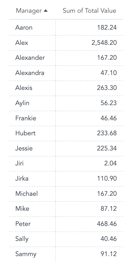
While each of the Total Values displayed are associated with a Manager, they are aggregated at the shop level. Matching values for two managers does not mean that they work in the same shop; Alexander and Michael are managers in different shops.
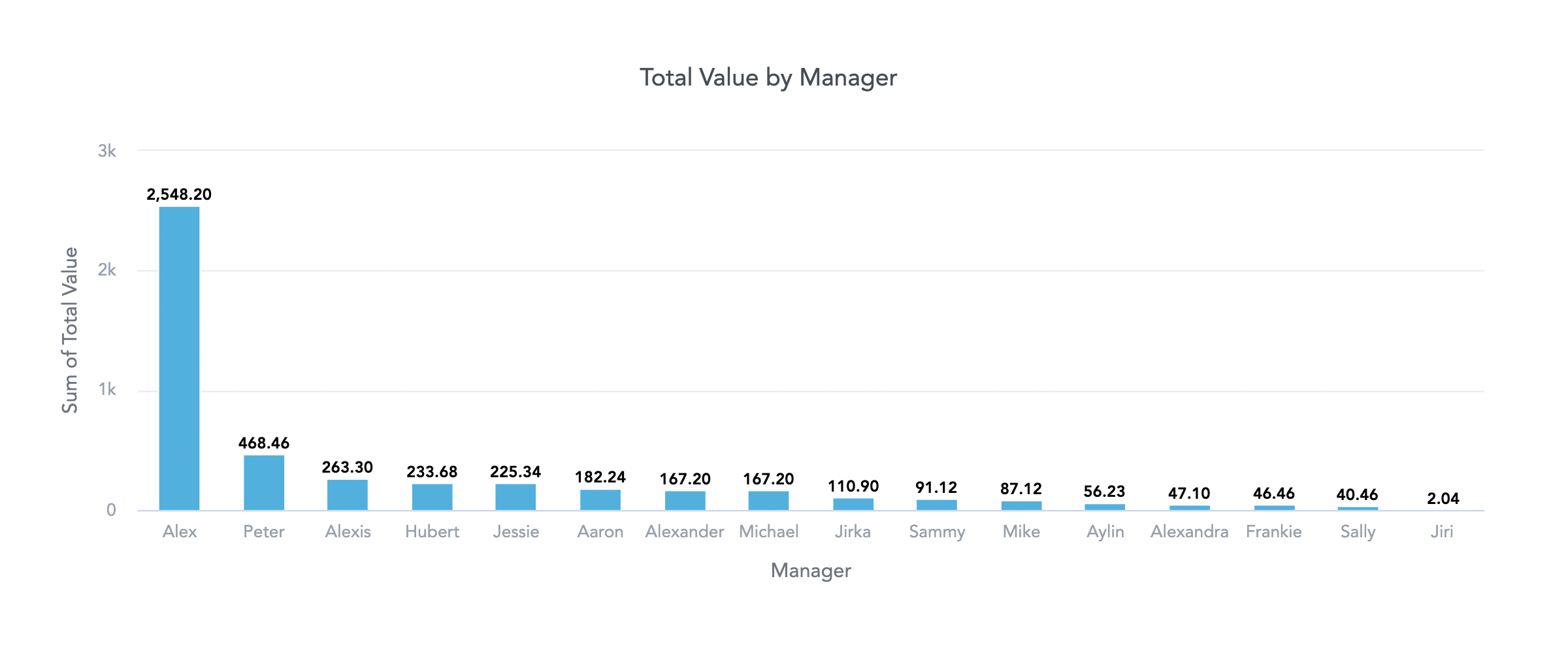
Switch to a different visualization to see who manages the top performing shops and the gross revenue earned by each manager’s shop.
Example 3 - Advanced explicit lifting
You can also count the average time that elapses between customers’ first two transactions.
Use explicit lifting to lock Transaction Date at the individual transaction level with the BY keyword. You can then calculate the difference between the transaction dates for each shopper. This displays the length of time for each shopper, as well as the average for the time elapsed between transactions across all shoppers.
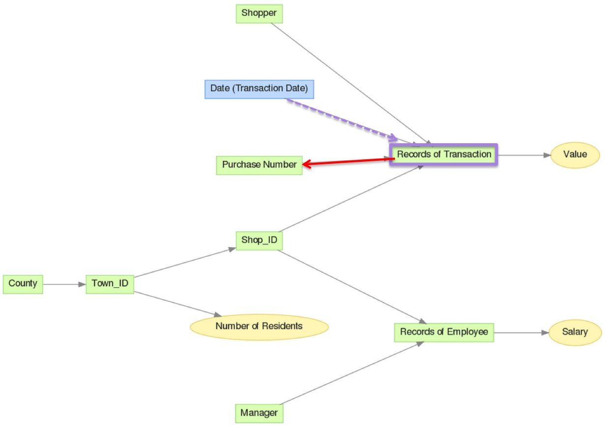
First, you must count the dates of the transactions. Select the date values of the various transactions, no aggregation is necessary.
SELECT Date (Transaction Date) BY Records of Transaction
To find out whether an aggregation function is necessary in an expression, visualize the process you want to carry out in the LDM from the project:
| Traversal direction | Required aggregation |
|---|---|
| Moving along a left-to-right arrow | This is explicit lifting. It requires no aggregation. |
| Moving along a right-to-left arrow | This is aggregation. It requires an aggregation function. |
Next, create two metrics that reference the original Transaction date lifted metric:
- A metric that filters the first purchase dates
- A metric that filters the second purchase dates
SELECT MAX(Transaction date lifted) WHERE Purchase Number = 1
SELECT MAX(Transaction date lifted) WHERE Purchase Number = 2
These metrics aggregate Transaction date lifted with a MAX function to filter it by purchase number. The reason are:
- SUM works if there is only one value in the data that corresponds to having a Purchase Number = 2. If there are multiple values where Purchase Number = 2, the metric double-counts values.
- AVG closely resembles the intention of the metric. However, AVG takes longer to calculate.
Finally, create a metric that computes the difference between the purchase date metrics. Then you can break the final result down by Shopper, which is the report-level attribute.
SELECT AVG(Second purchase date - First purchase date)
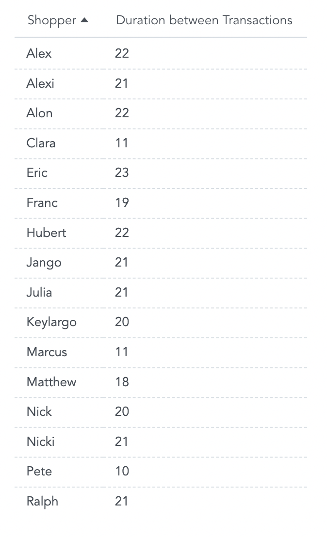
The resulting report shows duration between first and second visits broken down by the Shopper attribute.
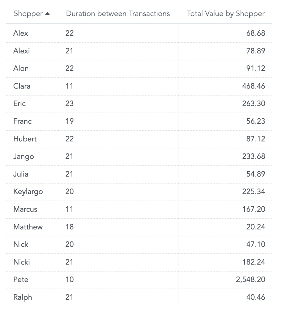
Adding the Total Value metric to the report (SELECT SUM(Value)) to look for correlations in duration between initial transactions and total amount spent.
To find the average duration between the first two transactions across all shoppers, modify the metric and remove all report attributes:
SELECT AVG((SELECT Second purchase date - First purchase date BY Shopper))