Analyzing Change with Historical Data (Snapshotting)

Analyzing the latest data and changes in GoodData is easy. This article uses a sales scenario but you can use it analyze your help desk, quality control or engineering and development data.

This article introduces the analytic technique called snapshotting. In the following scenario, you will work with the concepts of opportunities, sales stages, and change.

Sales Analytics

Sales Analytics is all about sales opportunities that are generated by your business activities. Each opportunity has a status that describes if the opportunity is Open (Pipeline), Won (Revenue), or Lost (Lost Revenue).

In this article, we try to answer a typical sales question: “What was the pipeline at the beginning of this quarter and how it has improved since then?”

Snapshotting Basics

To answer that question, you will use a technique called snapshotting. The key idea is that we keep transferring all opportunities from your CRM to GoodData every week (or day or month - it depends on your requirements). We call the weekly set of opportunities a snapshot. Each snapshot is associated with a date and an unique ID.

So if we have a project that accumulates snapshots for 118 weeks, most of our opportunities will be duplicated 118 times in the project. Few of them that have been created after we started snapshotting have less than 118 versions. Each version is associated with a snapshot date (perhaps Monday of each week) and the snapshot ID. It is very beneficial to use snapshot IDs in sequence without gaps. We can then simply identify previous/next snapshots as the current ID minus/plus one.

Here is the first catch. A simple SELECT SUM(Amount) WHERE Status = Open metric measures your pipeline returns a number that is roughly 118 times higher than what we expect. This is because we are adding up all ten versions of each opportunity. Instead, we can define metric that shows the total amount for individual snapshot only:

Pipeline [118 weeks ago]:

SELECT SUM(Amount) WHERE Status = Open AND SnapshotId = 1

Pipeline [Now]:

SELECT SUM(Amount) WHERE Status = Open AND SnapshotId = 118

However, you will need a new metric next week and another one week after next week. A metric that returns the total amount for the last snapshot would be handy. Let us start creating such a metric with identifying the last snapshot:

Snapshot [Most Recent]:

SELECT MAX(SnapshotId)

This definition sounds easy enough, however, it has certain problems. Imagine that you fired a Sales Representative John during the snapshot 25. We kept all opportunities that he has closed associated with him and re-associated all open opportunities to other sales guys.

Now if we break down the Snapshot [Most Recent] metric by the SalesRep, we will see that the metric returns 118 for all Sales Reps except John who gets the Snapshot [Most Recent] = 25. This is problem because we would compute our total on the snapshot 25 for John and on the snapshot 118 for everybody else. We need to improve the definition of the Snapshot [Most Recent] metric:

Snapshot [Most Recent]:

SELECT MAX(SnapshotId) BY ALL IN ALL OTHER DIMENSIONS WITHOUT PARENT FILTER`

This metric returns the MAX snapshot regardless any dimensions. The last snapshot (= 118) for all Sales Reps including John, for all regions, for all Products etc. When you add the BY ALL IN ALL OTHER DIMENSIONS statement to your metric it returns the grand total (MAX) of all the time and all dimensions. It returns a constant.

What is the WITHOUT PARENT FILTER clause for? Imagine that you place the metric into a report that contains the SalesRep = John filter. Applying this filter would lead to the same troubles that we’ve eliminated with the BY ALL IN ALL OTHER DIMENSIONS. The WITHOUT PARENT FILTER clause simply ignores the higher level filters.

Then we can use the Snapshot [Most Recent] metric in our pipeline metric and get the latest amount this way:

Pipeline [Now]:

SELECT SUM(Amount) WHERE Status = Open AND SnapshotId = Snapshot [Most Recent]

Similarly we can compute the pipeline for the first snapshot (the oldest one). The metric is:

Snapshot [Oldest]:

SELECT MIN(SnapshotId) BY ALL IN ALL OTHER DIMENSIONS

and use it in the following pipeline metric:

Pipeline [Oldest]:

SELECT SUM(Amount) WHERE Status = Open AND SnapshotId = Snapshot [Oldest]

Measuring Pipeline Change in a Quarter

The oldest and the most recent snapshots are great but we want something slightly different. We want to compute the pipeline for the first and the last snapshot in a quarter. We can achieve this by following metric definitions:

Snapshot [First in Period]:

SELECT MIN(SnapshotId) BY ALL IN ALL OTHER DIMENSIONS EXCEPT SnapshotDate WITHOUT PARENT FILTER

Snapshot [Last in Period]:

SELECT MAX(SnapshotId) BY ALL IN ALL OTHER DIMENSIONS EXCEPT SnapshotDate WITHOUT PARENT FILTER

Let’s focus on the BY ALL IN ALL OTHER DIMENSIONS Except statement. Using this concept it allows you to compute total MAX/MIN of SnapshotId regardless any dimension but with exception of the specific attribute. The exception is an attribute after the EXCEPT expression. So the resulting number is not going to be a constant anymore. It will depend on the value of the SnapshotDate. In other words this metric returns the maximum SnapshotId for the SnapshotDate period.

If you put the metrics above to a report with the Snapshot Quarter, you will see the first and the last snapshot ID that we have for each quarter. See the report below:

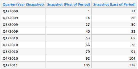
So then the pipeline at the beginning of a period is:

Pipeline [First in Period]:

SELECT SUM(Amount) WHERE Status = Open AND SnapshotId = Snapshot [First in Period]

And the latest and greatest pipeline number is:

Pipeline [Last in Period]:

SELECT SUM(Amount) WHERE Status = Open AND SnapshotId = Snapshot [Last in Period]

Now you just put these two metrics into a report with the Snapshot Quarter and you’ll get the pipeline at the beginning of each quarter and the last known pipeline each quarter.

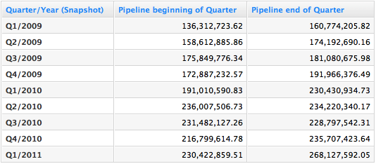
Depending on your needs, you can divide or subtract these numbers to get the absolute or relative growths.